
Even at high sample rates, standard PCM audio ‘smears’ important timing information. A new digital format, MQA, promises vastly improved time-domain accuracy — without the huge file sizes.
The goal of any music recording/replay system is to capture the sound of an artist’s performance and reproduce it accurately for the listener. Of course, this is much easier said than done, and the practical achievement of such an ostensibly simple requirement is a challenge which has consumed the audio industry for over a century. However, British start-up company MQA are promoting a genuinely groundbreaking system that, they claim, exceeds the sound quality of all current hi-res formats, without requiring high data rates and while remaining fully backwards-compatible with the legacy 16-bit/44.1kHz format!
Of particular interest from the audiophile perspective is the assertion that this new system achieves an astonishingly precise time-domain performance. However, it’s the way it addresses the pragmatism of modern music consumerism that makes it a strong candidate as the leading future consumer format for streaming and downloading ‘high-resolution’ audio — and that’s why it is something that Sound On Sound readers need to know about.
Before I explore the detail of this ingenious new system, though, we need to revisit some digital audio theory to fully understand the ways in which the new format is advancing across previous technological boundaries. As we all know, the possibilities of analogue technology had largely been exhausted by the 1990s, and while noise, distortion, and wow and flutter were reduced almost to the point of inaudibility, they could never be removed completely. Modern digital audio is not only far more cost-effective than the best of analogue, it also enjoys greatly improved performance on the parameters mentioned above. However, the inherent time-domain artifacts associated with Nyquist filtering deny total audio perfection from us!
Tripod Of Audio Quality
Audio quality can, perhaps, be defined in three interrelated ways: dynamic range, frequency bandwidth and temporal precision. Analogue electronics have long since met the dynamic range requirement, although none of the mechanical analogue recording formats could deliver 120dB. In the digital domain, dynamic range is determined by the word length, and 16 bits with noise-shaped dithering easily meets the perceptual dynamic range requirements for any practical domestic listening environment. For professional work, 24 bits is more than sufficient for source recording, and although it is true that (post-production) signal processing often requires greater resolution, that is simple to achieve with well-known DSP number-crunching techniques, such as ‘floating-point’ calculations. So, we can tick the dynamic range box.
Audio bandwidth varies considerably between different analogue systems. For example, the low end is necessarily curtailed for vinyl records, and the high end for FM radio. But for most analogue systems (including microphones and loudspeakers) the roll-offs at both frequency extremes are usually relatively gentle, and with small group delays or phase shifts. In contrast, the bandwidth of conventional digital audio systems is defined by the practicalities of the ‘brick-wall’ anti-aliasing and reconstruction filtering, which is directly related to the sample rate. While the use of 44.1 or 48 kHz sampling rates potentially compromises the audible bandwidth slightly, the double- (88.2/96kHz) and quad-rate (174.4/192kHz) formats are blameless in that respect, yet the filtering may still impose unwanted audible side-effects. Of course, other formats exist with even higher sample rates. So, we can tick the bandwidth box too.
Most of us think of audio equipment performance in terms of the frequency domain. When we talk of equalisation we think of how the amplitude changes at different frequencies, for example, and when we compare equipment specifications we often rely on the frequency response as an arbiter of quality. However, this is only half the story, the other half being the time-domain performance. This is a much more relevant concept when considering digital systems, albeit one which is far less natural and intuitive for most of us.
While phase shifts and group delays are often considered when defining audio quality, temporal precision is rather less well understood, and has been largely ignored until relatively recently. However, it has been known about in some sense since the work of Von Békésy back in 1929. He was investigating the acuity of human hearing in identifying sound source directions, and his work suggested that the ear can resolve timing differences of 10µs or less. This was extended in 1976 when Nordmark’s research indicated an inter-aural resolution of better than 2µs! More recent international research confirms that the human auditory system can resolve transient timing information down to at least 8µs, too.
To put this in context, simple maths indicates that a sinusoidal period of 8µs represents a frequency of 125kHz — but no one is suggesting the perceptual bandwidth of human hearing gets anywhere near that! Entirely different ear and brain functions are involved in detecting a signal’s arrival timing and its frequency content, possibly in much the same way that the ‘rod’ cells in the eye detect brightness or luminance, while only the ‘cone’ cells detect colour. So the established auditory bandwidth of around 20kHz remains broadly accepted as fact, and a secondary system is presumed to be involved in detecting signal transients with remarkably precision. Perhaps one of the reasons we have seen a trend towards higher and higher sample rates in ‘hi-res’ audio equipment over recent years is because higher sample rates inherently improve the ‘temporal precision’ to some degree.
Impulse Responses
Historically, our analysis and assessment of audio equipment has been based primarily on its frequency-domain performance. That emphasis has influenced the ubiquitous use of linear-phase ‘brick-wall’ filters in digital equipment, since they offer a convenient way of achieving a near-perfect frequency-domain characteristic (with negligible ripple in the pass-band). However, recent research proposes that the filters’ time-domain behaviour should be given greater priority, especially in light of the ear’s apparently extraordinary temporal resolution mentioned earlier.
") Figure 1: A typical brick-wall filter’s impulse response for a 48kHz digital system. Note the pre- and post- ringing extending considerably from the central impulse. (Shown with a linear amplitude scale.)
Figure 1: A typical brick-wall filter’s impulse response for a 48kHz digital system. Note the pre- and post- ringing extending considerably from the central impulse. (Shown with a linear amplitude scale.)
When we use impulse responses to analyse the time-domain behaviour of a linear-phase filter, what we find is a response with significant pre- and post-ringing (see Figure 1).
The filters employed in a 44.1kHz or 48kHz system typically have ringing tails extending for several hundred microseconds before and after the main impulse. These ‘ringing tails’ act to spread out the signal’s energy over time — often referred to as ‘temporal blurring’ — and it is thought that our sense of hearing may be sensitive to this side-effect. It is also the case that pre-ringing, where sound energy builds up in advance of the sound’s actual starting transient, cannot possibly occur in nature. This could, therefore, be a particularly unnatural and undesirable artifact of existing digital technology.
Of course, the idea that these ringing tails are a ‘bad thing’ is not new, and converter manufacturers like dCS and Wadia (amongst others) have been offering alternative filtering schemes for many, many years. So what can be done to get rid of these impulse response tails? Well, there are several ways to reduce their duration, and the first and easiest is simply to employ higher sampling rates — which is possibly why some listeners claim that existing ‘hi-res’ audio formats sound more natural. However, this approach is subject to rapidly diminishing returns above 96kHz: the audio data rate grows enormously and impractically, for only moderate reductions in the filter ringing duration.
") Figure 2: A typical minimum-phase brick-wall filter’s impulse response for a 48kHz digital system. Note the absence of pre-ringing, but stronger and longer post-ringing. (Shown with a linear amplitude scale.)
Figure 2: A typical minimum-phase brick-wall filter’s impulse response for a 48kHz digital system. Note the absence of pre-ringing, but stronger and longer post-ringing. (Shown with a linear amplitude scale.)
Another approach, which has become quite popular in recent years, is to use a ‘minimum-phase’ filtering scheme instead. This technique removes the unnatural pre-ringing tail completely while maintaining the required ‘brick-wall’ frequency response. However, the inescapable compromise is that the pre-ring energy effectively re-appears in the form of a louder and longer post-ring tail (see Figures 2 and 3). So although this approach results in a more ‘real-world’ impulse response, with no unnatural pre-echoes, the same overall temporal blurring effect remains.
 and minimum-phase (green) filters shown above, but this time as the energy or power distribution with a logarithmic amplitude scale. Note that the time offset between the main impulses is due to the nature of the FIR hardware used to implement the two filters and is typical of real-world executions.") Figure 3: This graph offers an alternative view of the linear-phase (red) and minimum-phase (green) filters shown above, but this time as the energy or power distribution with a logarithmic amplitude scale. Note that the time offset between the main impulses is due to the nature of the FIR hardware used to implement the two filters and is typical of real-world executions.
Figure 3: This graph offers an alternative view of the linear-phase (red) and minimum-phase (green) filters shown above, but this time as the energy or power distribution with a logarithmic amplitude scale. Note that the time offset between the main impulses is due to the nature of the FIR hardware used to implement the two filters and is typical of real-world executions.
It is a fact that the duration of a filter’s impulse response is directly related to the steepness of the filter’s slope, so perhaps a better approach would be to use much gentler filters — something like a third-order (18dB/octave) Butterworth (minimum-phase) filter, for example, which is commonly employed in analogue systems without complaint! However, if we were to try to do that within a conventional digital system, we would need an extraordinarily high sampling rate to ensure adequate separation between the audio pass-band and the Nyquist limit, to avoid aliasing problems. Sony’s Direct Stream Digital (DSD) system used in the SACD format takes a long stroll in this direction, but to make the data rate practical, it operates with a one-bit PCM format which is difficult to process and requires very heavy noise-shaping to achieve a workable signal-noise ratio in the audio pass-band. So it’s still not an ideal solution.
 There are already a number of MQA-enabled players available from manufacturers such as Bluesound and Pioneer.
Apodization
An ingenious way of enjoying the benefits of a gentler filter slope within an existing digital system with a sensible sample rate is derived from a technique employed in radio astronomy, amongst other applications. The edge of a parabolic dish antenna creates a sharp discontinuity in its performance, causing the equivalent of diffraction rings or ripples which ‘blur’ the wanted celestial images. This discontinuity effect, called the Gibbs Phenomenon, is well known in theoretical maths and affects many applied sciences. In radio astronomy, engineers deliberately ‘taper down’ the contributions from the outer parts of the parabolic dish to reduce this effect: a procedure referred to as ‘apodization’.
Research into how apodization could be usefully employed in the context of digital audio systems was published in 2004 by Peter Craven, who is well known for his work with the late Michael Gerzon in developing the Soundfield microphone and Ambisonics, amongst other things. The first practical realisation of this work was when British hi-fi manufacturers Meridian introduced an ‘apodizing filter’ DSP process into some of their products. (It may also be of interest to know that various forms of apodizing filter are routinely employed in spectral analysis tools, a common form being the Hann window function).
. This potentially results in aliasing (in the green shaded area) but this can also be removed by apodization. (Shown with a linear amplitude scale.)") Figure 4: The solid red line shows the apodizing filter frequency response, designed for a flat audio pass band and maximum attenuation in the transition-band region of typical brick-wall filters. The green line shows the frequency response of a typical ‘half-band’ brick-wall filter (which only manages 6dB attenuation at the Nyquist frequency). This potentially results in aliasing (in the green shaded area) but this can also be removed by apodization. (Shown with a linear amplitude scale.)
Figure 4: The solid red line shows the apodizing filter frequency response, designed for a flat audio pass band and maximum attenuation in the transition-band region of typical brick-wall filters. The green line shows the frequency response of a typical ‘half-band’ brick-wall filter (which only manages 6dB attenuation at the Nyquist frequency). This potentially results in aliasing (in the green shaded area) but this can also be removed by apodization. (Shown with a linear amplitude scale.)
In simple terms, the apodizing filter is designed to impose a relatively gentle cutoff slope above the wanted audio pass-band, as shown in Figure 4, yet still achieve full attenuation well before the Nyquist limit. This approach is clearly only practicable, though, where the sample rate is significantly higher than the required audio bandwidth (ie. for 96kHz sample rates and above).
Every digital audio chain involves a cascade series of filters — such as anti-alias, band-limiting (if sample-rate conversion is involved), and reconstruction filters — and the overall system’s frequency response is the product of their individual responses. However, in the time-domain, the overall impulse response of the chain is the convolution of their individual responses: and, usefully, the convolution process allows a cascade series of filters to elicit a shorter impulse response than that of any individual filter in the chain! Consequently, an apodizing filter can be designed to almost completely remove the pre- and post-ringing tails associated with a chain of conventional linear-phase filters. This might seem completely counter-intuitive, but as Figure 5 reveals, it’s true nonetheless!
 with the same chain corrected with an apodizing filter (blue). Note the almost complete removal of pre- and post-ringing tails, and greatly reduced temporal-smearing. (Note the linear amplitude scale.)") Figure 5: This compares the typical impulse response of a digital audio chain using conventional linear-phase brick-wall filters (red) with the same chain corrected with an apodizing filter (blue). Note the almost complete removal of pre- and post-ringing tails, and greatly reduced temporal-smearing. (Note the linear amplitude scale.)
Figure 5: This compares the typical impulse response of a digital audio chain using conventional linear-phase brick-wall filters (red) with the same chain corrected with an apodizing filter (blue). Note the almost complete removal of pre- and post-ringing tails, and greatly reduced temporal-smearing. (Note the linear amplitude scale.)
Moreover, a single apodizing filter can be designed to compensate for the time-domain responses of any number of linear-phase brick-wall filters in the signal path, and without needing to know their exact number or precise types. This means that apodization is equally effective whether applied to a current conventional digital signal chain, or to an archive of historical digital recordings.
As an aside, it is interesting to note that this is not the first time that advancing technology has improved the quality of archive material retrospectively! The size of the magnetic gap in an analogue tape machine’s head determines the upper frequency limit for replay, but it does not affect the recording process in the same way. The engineering of tape heads in the 1940s and ’50s was such that they all had relatively wide gaps and thus a limited replay high-frequency response, but when it became possible to manufacture tape heads with very narrow gaps in the late ’60s it was discovered that archived early tape recordings had actually captured a very wide audio bandwidth that easily matched or exceeded the capabilities of the newer narrow-gap heads. Consequently, recordings from the ’40s and ’50s could be auditioned with a full audio bandwidth for the first time!
Sampling Evolution
Although apodization is a very clever way of improving the time-domain performance of legacy digital systems, in an ideal world we shouldn’t need to ‘fix the system’: it would be much better if the system’s native impulse response was already ‘perfect’. In trying to define ‘perfect’, perhaps a valid answer would be an impulse response similar to that of an acoustic sound wave passing through a few metres of air, for that would then be a genuinely ‘transparent’ digital system. So, given a free design hand, is there a way of creating a digital audio system with a very short and natural impulse response of this type? Astonishingly, the answer appears to be yes!
The familiar Nyquist-Shannon Sampling Theorem stems from the development of ‘Information Theory’ in the early 1920s. So it’s a very well established and thoroughly proven theorem which, in addition to guiding the development of digital audio systems for the last 40 years, has been employed widely across countless other aspects of everyday science and technology. However, the use of band-limited signals, brick-wall filters, Fourier transforms, and Sinc-function reconstruction kernels — all of which the theorem has guided us to employ — is not, technically, mandatory. There are other approaches that don’t suffer the same uncertainty between time and frequency information that is inherent in the Fourier model... and developments in advanced mathematics over the last 15 years or so (particularly in relation to Wavelet Theory and complex image processing) have led to many momentous advancements in both the fundamental concepts and the practical techniques of sampling theory.
Of particular interest are new techniques which essentially discard brick-wall anti-alias filtering as we currently know it, and employ new forms of sampling and reconstruction kernels that can resolve transient signal timing with extraordinary resolution, even conveying positional time differences that are shorter than the periods between successive samples! This seems counter-intuitive but it is possible if, instead of using traditional adjacent rectangular sampling periods, a series of overlapping and time-weighted triangular sampling kernels are used (see Figure 6). Even better results are possible using higher-order ‘B-spline’ kernels, which allow both the position and intensity to be identified of two or more separate pulses occurring within the same sampling period!
 effectively integrates the area of the transient to determine its intensity within the sampling period. However, the sample value will not change regardless of where within the sampling period the transient occurs. Consequently, this arrangement cannot identify the precise position in time of a transient pulse within the sampling period. However, by using overlapping triangular sampling kernels (bottom), both the time and intensity of a transient pulse can be recovered. (Note: this diagram assumes no anti-alias filtering, since the pulse is clearly of much shorter duration than the sample period, breaking the Nyquist rules — see main text!)") Figure 6: A conventional rectangular sampling kernel (top) effectively integrates the area of the transient to determine its intensity within the sampling period. However, the sample value will not change regardless of where within the sampling period the transient occurs. Consequently, this arrangement cannot identify the precise position in time of a transient pulse within the sampling period. However, by using overlapping triangular sampling kernels (bottom), both the time and intensity of a transient pulse can be recovered. (Note: this diagram assumes no anti-alias filtering, since the pulse is clearly of much shorter duration than the sample period, breaking the Nyquist rules — see main text!)
Figure 6: A conventional rectangular sampling kernel (top) effectively integrates the area of the transient to determine its intensity within the sampling period. However, the sample value will not change regardless of where within the sampling period the transient occurs. Consequently, this arrangement cannot identify the precise position in time of a transient pulse within the sampling period. However, by using overlapping triangular sampling kernels (bottom), both the time and intensity of a transient pulse can be recovered. (Note: this diagram assumes no anti-alias filtering, since the pulse is clearly of much shorter duration than the sample period, breaking the Nyquist rules — see main text!)
Not surprisingly, though, the very elaborate mathematics that prove and explain all this are way above my comprehension level. I’ve read a lot of the relevant academic papers and patents, and although I understand most of the printed words individually, when formed into complete sentences they somehow become entirely meaningless to me! If you’re interested in investigating this further, I’ve listed some relevant AES papers and Meridian patents in the References box, but be warned: they aren’t easy reads, and appear to be deliberately incomplete or strategically vague in places.
Nevertheless, I believe these very advanced sampling techniques are already being employed in many non-audio fields, including medical imaging and military radar, so it’s only a matter of time before they find more mundane applications in the world of professional audio! And this is where the new MQA format becomes directly relevant.
The MQA Concepts
This ingenious new system appears to offer an interesting and practical step forward for digital audio. It is claimed that MQA does ‘no more harm’ to an audio signal than it would suffer in passing through a few metres of air, and that it exceeds the sound quality of all current hi-res formats without requiring high data rates, and while remaining fully backwards-compatible. In other words, it addresses not only the time-domain issues of legacy digital audio systems, but also some of the pragmatic realities of modern music consumerism. As such, this new scheme seems ideally placed to become a — if not the — leading future consumer format for streaming and downloading audio, for both high- and standard-resolution applications!
 Chairman and CEO of MQA is Bob Stuart, best known for founding hi-fi manufacturers Meridian Audio.
Bob Stuart (co-founder of Meridian Audio) and Peter Craven (independent researcher and consultant, Algol Applications Ltd) worked for more than five years to develop this technology, and it is now being marketed by an independent start-up company called MQA, of which Bob is chairman and CEO. The acronym stands for ‘Master Quality Authenticated’, and the concept was announced to the public in 2014. Since then it has caused a bit of a storm within the hi-fi press, but it hasn’t made much impact on the professional side of the industry until now.
However, MQA claim they are on the verge of breaking into the professional mainstream, as artists, record labels, mastering houses, and streaming/download content providers are starting to embrace the idea. Content providers, including Jay Z’s Tidal music-streaming service and the UK’s 7digital download service, have already signed up, along with Scandinavian classical download label 2L, Onkyo Music and HQM Store. A number of well-known hi-fi and professional equipment manufacturers have also released compatible hardware, or are in the process of developing MQA-compatible converters. The list so far includes the likes of Pioneer, Bluesound, Mytek, Onkyo and, of course, Meridian, and MQA say many more are actively investigating the possibilities with them.
Authentication
In essence, the MQA platform comprises three completely separate but equally important elements. The first, and the simplest to comprehend, is hinted at clearly by the name itself: MQA files incorporate a digital ‘signature’ securely buried within the audio data which is examined by the replay system’s MQA-compatible D-A converter. This examination provides authentication that the reconstructed audio file delivered to the consumer’s ears is exactly the same as that encoded and approved by the file’s author. in practice that typically means the artist’s or label’s mastering engineer, of course.
So, if the audio file has been up-sampled from a lo-res version, or doctored in any way at all — which is not uncommon for some supposedly hi-res audio download and streaming providers — it will not be recognised as a genuine MQA file. The intention is that, on detection of an untarnished file, an MQA replay system will display a label or light to confirm that the listener is hearing exactly what the artist approved for release. Obviously, this ‘authenticated quality’ feature is hoped to set MQA files apart from, and qualitatively above, other generic hi-res audio file formats in the marketplace.
Convenience
The second pillar of the MQA trilogy is a matter of convenience. Raw high-resolution audio files are inherently big, and that’s just not very convenient, especially if you want to stream hi-res audio files in real time to a portable device. Broadband and mobile connections may generally be getting faster and data allowances bigger but, even so, the prospect of streaming lots of hi-res audio is still not particularly attractive or practical for most of us.
Historically, of course, this problem has been circumvented through the use of data-reduction formats, but lossy codecs like MP3 and AAC defeat the whole purpose of ‘hi-res’ audio — it is quite sobering to think that the data rate of a 128kb/s MP3 file is 72 times smaller than that of a hi-res 24-bit/192kHz WAV file! The alternative lossless formats such as FLAC and ALAC can offer only relatively modest reductions in the amount of data being transferred, so aren’t really much help.
A major part of the hi-res data size problem is that the ‘information space’ of a high sample-rate linear PCM signal is largely wasted, since much of that encoding space is either empty or below the environmental noise floor (see Figure 7). In fact, only about one-sixth of the total information space contains relevant audio information!
 and mean noise spectra (blue) derived from a recording of the Guarneri Quartet playing Ravel’s String Quartet in F, second movement. Near-identical results are obtained regardless of the music genre, with the same declining peak level with frequency, and the same convergence of signal and noise in the 48-60 kHz region. At higher frequencies, noise will obscure any tonal high-frequency signals. Extensive analysis of all forms of music has shown that all relevant audio information can be contained within the yellow triangle.") Figure 7: A Shannon diagram showing the total coding space for a 24-bit/192kHz recording system, with the peak signal level (red) and mean noise spectra (blue) derived from a recording of the Guarneri Quartet playing Ravel’s String Quartet in F, second movement. Near-identical results are obtained regardless of the music genre, with the same declining peak level with frequency, and the same convergence of signal and noise in the 48-60 kHz region. At higher frequencies, noise will obscure any tonal high-frequency signals. Extensive analysis of all forms of music has shown that all relevant audio information can be contained within the yellow triangle.
Figure 7: A Shannon diagram showing the total coding space for a 24-bit/192kHz recording system, with the peak signal level (red) and mean noise spectra (blue) derived from a recording of the Guarneri Quartet playing Ravel’s String Quartet in F, second movement. Near-identical results are obtained regardless of the music genre, with the same declining peak level with frequency, and the same convergence of signal and noise in the 48-60 kHz region. At higher frequencies, noise will obscure any tonal high-frequency signals. Extensive analysis of all forms of music has shown that all relevant audio information can be contained within the yellow triangle.
Looking at the diagram above, several things become apparent. First, a sample rate greater than 96kHz is required to encode all of the musically relevant information (as well as being important in helping to minimise temporal blurring). Second, everything above about 50kHz is just noise. Third, within the base-band area below 24kHz, the range from peak signal level to noise floor is within the dynamic range that can be captured with a properly dithered 18-bit system. And last but most important, the musical information only occupies a fraction of the total information space, with the greatest dynamic range at low frequencies and the smallest at ultrasonic frequencies. As linear PCM formats treat every part of the information space as being equally vital, when clearly that’s not the case, the system is inherently grossly inefficient.
Taking all of these things into account, the MQA format approaches the efficiency problem from the standpoint of matching the encoding format to the capabilities and requirements of the human auditory system, focusing on the relevant and wanted information without wasting resources on the irrelevant aspects.
To meet these challenges, MQA uses the sophisticated data-reduction strategy described in the ‘Music Origami’ box. This, in effect, ‘folds’ the relevant high-frequency audio information back into the noise-floor region of the base-band audio signal — but in such a way that it can be extracted and reconstructed for lossless replay. The sample rate of an MQA file is always based on that of its source material, so original material at 88.2, 176.4 or 352.8 kHz would be encoded as a 44.1kHz MQA file, whereas material starting out with 96, 192 or 384 kHz sample rates would be encoded as an MQA file at 48kHz. (Maintaining the base sample rate for each format is essential, as any sample-rate conversion processes would compromise the system’s time-domain performance.)
However, regardless of the MQA file’s actual sample rate, the streaming data rate is a little over 1.5Mb/s, and MQA files are fully backwards-compatible with legacy 16/44.1 systems, too — so MQA files can be transferred or used anywhere, and on anything, that can handle conventional 24- or 16-bit 44.1 or 48 kHz WAV files.
Lords Of The Time Domain
The third and final pillar of the MQA system is the format’s radically improved time-domain performance, which really sets it apart from all previous digital audio systems. The company have established a challenging target of delivering a perceptual time smear of about 10µs for existing digital recordings (it’s around 100µs for a conventional 24/192 system), with the aim of achieving an astonishing 3µs for newly recorded material. To put some qualitative numbers on all this, 10µs of time smear is roughly equivalent to that encountered by sound waves passing through 10m of air.
 against a conventional 24/192 linear-phase digital system (red). Note the amplitude scale here is logarithmic, not linear, which accounts for the very different visual presentation of the pre and post-ringing tails of the linear-phase system.") Figure 12: This graph compares the impulse response of an MQA system in a complete end-to-end configuration (blue) against a conventional 24/192 linear-phase digital system (red). Note the amplitude scale here is logarithmic, not linear, which accounts for the very different visual presentation of the pre and post-ringing tails of the linear-phase system.
Figure 12: This graph compares the impulse response of an MQA system in a complete end-to-end configuration (blue) against a conventional 24/192 linear-phase digital system (red). Note the amplitude scale here is logarithmic, not linear, which accounts for the very different visual presentation of the pre and post-ringing tails of the linear-phase system.
However, this exacting level of time-domain performance is only possible when MQA is employed as a complete end-to-end system, encompassing both the original A-D sampling and encoding within the mastering process, as well as the consumer access and decoding stages. In this way, and with the implicit and precise knowledge of all digital filtering processes involved in the chain, the system’s overall impulse response can be made almost perfect. For example, MQA claim that the total impulse-response duration is reduced to about 50µs (from around 500µs for a standard 24/192 system), and that the leading-edge uncertainty of transients comes down to just 4µs (from roughly 250µs in a 24/192 system).
Given these specifications, it seems clear that the MQA format potentially raises time-domain performance of digital systems to a level that not only matches, but actually exceeds that of traditional analogue equipment — including the time-domain performance of conventional studio microphones! It is already the case that the full MQA mastering process corrects for the group delays (phase response) inherent in specific analogue tape recorders used to replay legacy archive tapes. In the future it could even correct for the time-domain behaviour of studio mics and mixing consoles too, getting the listener even closer to the actual sound created in the studio!
MQA Decoding
As already mentioned, in its folded state, the streaming audio file has as typical bit rate around 1.5Mb/s (and never more than 2Mb/s, even in extremis). This is within the capabilities of a 3G mobile data service, and it presents no challenge at all for a 4G data link. Consequently, the MQA format satisfies the claim that it offers convenient and practical downloading and audio streaming for genuine hi-res audio files.
An integral element of MQA’s design is that even in its ‘folded’ and undecoded state, the 44.1kHz or 48kHz MQA audio file can still be replayed by any legacy device — even those limited to 16-bit resolution — without any audible artifacts. This is because the high-frequency content is buried within the noise floor, and the core audio is contained (and properly dithered) within the most significant 16 bits. A significant commercial benefit of this is that download and streaming services don’t need multiple file inventories to satisfy different end-user requirements. Moreover, the benefits of the MQA system’s avoidance and correction of temporal blurring will still be partially apparent even when replayed on standard legacy base-rate players.
 Figure 13: This graph shows both the impulse and frequency responses of the MQA system in a complete end-to-end configuration. Note the dual scales.
For the hi-res consumer, if an MQA file is presented to an MQA-compatible converter (and assuming the data passes the authentication check), the original origami process is completely reversed to fully reconstruct the desired 24/192 output signal, and with an immaculate frequency and impulse response as seen in Figure 13. With such a sophisticated system, you might expect the decoding requirements to be rather challenging and difficult to implement, but surprisingly, the decoder technology is not all that demanding at all. It’s really just a matter of some additional digital filtering software to correct for the D-A hardware’s specific time-domain characteristics, as well as to conform to the requirements of MQA’s encoding process, and the ability to detect and interpret the buried authentication and system metadata.
As many current high-end DACs are already software-controlled, at least some high-end products could in theory be upgraded for MQA compatibility through a simple firmware upgrade; this is certainly the case for some of Meridian’s own products. I suspect, though, that the majority of manufacturers will prefer to release brand new MQA-compatible hardware converters.
Professional Applications
For the professional market, MQA decoding and encoding could be achieved very conveniently and practically with a bespoke DAW plug-in, and MQA are already working on releasing a professional decoder plug-in later this year. However, the substantial temporal benefits of the MQA format are only achieved with total control over the complete end-to-end encode/decode process, so any MQA encoder plug-in would need to be user-configurable to account for the time-domain behaviour of the specific A-D converters being used and, ideally, that of any analogue hardware in the chain, too. This is not impossible, but it would be a very complex task that would require a lot of testing of legacy hardware converters to establish a workable time-domain database. So, perhaps MQA-compatible hardware A-D converters would be a more practical first step... and various manufacturers are already working on that.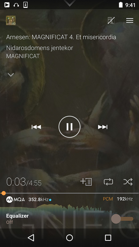
 One of the selling points of MQA is 'authentication': when the MQA logo appears, as in these screen captures from Onkyo and Pioneer players, listeners can be certain they are listening to the audio file as the artist and mastering engineer intended.
Conclusion
From the marketing and user-convenience points of view, MQA seems to tick all the compatibility, convenience and practicality boxes for both consumers and vendors, and it appears to be able to deliver an astonishing level of time-domain performance never before seen in conventional digital systems. The format’s file authentication and ‘music origami’ data-reduction processing are both extremely clever and highly pragmatic, too. Whether or not MQA becomes the new streaming and download format of choice, only time will tell, but it certainly has a great deal in its favour.
The obvious final question, though, must be: does it really sound better than conventional hi-res digital recordings? I’d like to be able to give a confident and definitive Yes in response... but I’m not sure I can just yet. That’s not because I wasn’t impressed with what I heard, but because I wasn’t sufficiently familiar either with the Meridian replay systems used to audition a variety of MQA recordings, or the source material itself, to form a totally confident opinion.
However, what I can say with confidence is that my initial impression of what I heard was of a generally more believable and realistic sound stage, with instruments and ensembles appearing more vibrant and genuinely three-dimensional in a way which exceeded anything I’ve heard with conventional hi-res audio on high-quality monitoring systems. Everything was located within very natural-sounding and acoustically defined spaces, and transient-rich instruments — cymbals and drums in particular — became noticeably more tangible. Overall, I think there was just more innately meaningful positional information coming from the speakers. The hi-fi world often describes the benefit of the latest high-end product costing more than my first house as “like lifting a veil”, and here, I think that word-picture is actually quite apposite!
Comparing MQA and conventional hi-res files wasn’t a blatant ‘night and day’ kind of difference. Whatever their limitations, 24/96 or 24/192 files do unquestionably deliver an extremely high sound quality. Nevertheless, the MQA format does appear to bring about a subtle but worthwhile improvement in perceived realism, and one which might become more recognisable and significant as the listener perhaps learns to stop subconsciously compensating for the intrinsic time-domain imperfections of ‘legacy’ digital technology and starts to listen au naturel once more!
I was left with the impression that my brain was having to do a lot less guesswork when analysing what I was listening to and what was making the sound. Over extended listening sessions, this might translate into far lower levels of listener fatigue, too... but then maybe it was just because Meridian’s top-of-the-range DSP8000SE active digital speakers, positioned carefully in a fully treated professional listening room, are stunningly good loudspeakers, with very tidy time-domain responses themselves!
We hope to be able to explore this MQA technology in a more practical way in the not too distant future, and specifically from the perspective of professional mastering and source recording. Watch this space!
Music Origami
 Figure 8: This is the same Shannon diagram as Figure 7, but with the regions encoded by different sample rates colour-coded. Base sample rates encode the brown area A, while double-sample-rate systems extend that to include the red region B. Quad sample rates extend the bandwidth to include the region C. The vast majority of wanted audio is contained within region A, with a significant amount in region B, but the audio content in region C is negligible.
The data-reduction process by which high-resolution audio is transmitted at modest data rates is described in the MQA literature as ‘music origami’, and that is quite a descriptive term for what’s going on in the two-stage ‘encapsulation’ process (Figure 9). As we know, the core information in any music recording is contained in the frequency region between, say, 5Hz to 22kHz — basically the material that we would record on a conventional CD (marked ‘A’ in the diagrams).
In the region above that, from 22kHz to 44kHz (or 48kHz in the case of a 192kHz sampled system), there is still a small amount of musical information above the noise floor (B), and that should be retained for a high-resolution audio system as it’s considered relevant. In a high sample-rate system running at, say, 192kHz, there is also a third region, from 48 to 96 kHz (C), although that contains only environmental and electronic noise.
 Figure 9: MQA’s ‘music origami’ starts by folding or ‘encapsulating’ the top half of the original 24/192 signal using lossy data reduction into the area below the noise floor of the B region, and the sample rate is reduced to 96kHz.
MQA’s music origami trick starts by ‘folding’ from 192 to 96 kHz, in effect remapping the highest frequency region (48-96 kHz) described above (C) into the area below the noise floor of the middle (B) region (around -130dBFS, between 24-48 kHz). This is not conventional downsampling; the process is referred to as ‘encapsulation’ and is technically a form of lossy data reduction. However, this is deemed acceptable because there is generally no relevant audio information here, just noise: it’s purely about being able to maintain the original high sample rate when decoded.
The observant reader might notice that if some relevant audio signal is still present in this C zone, as illustrated by the tip of the yellow triangle in the diagram above, the first stage of spectral folding will cause some aliasing immediately below 48kHz. However, whereas conventional sample-rate conversion would employ an anti-alias filter to prevent this, the MQA encapsulation process does not, since doing so would cause unwanted timing blur. Thankfully, any aliased elements will always be at a much lower level than the audio elements within the B region, and extensive testing has shown this aliasing to be completely inaudible.
 and buries it losslessly under the noise floor of the A region, with the final format arranged as in Figure 11.") Figure 10: The second origami fold takes the data in the B region (which already includes that of the C region) and buries it losslessly under the noise floor of the A region, with the final format arranged as in Figure 11.
Figure 10: The second origami fold takes the data in the B region (which already includes that of the C region) and buries it losslessly under the noise floor of the A region, with the final format arranged as in Figure 11. Part two of the process (Figure 10) involves genuinely lossless data reduction to store the middle (B) region’s audio information (now including the encapsulated C region too, of course) into the area underneath the noise floor of the base-band A region below 22/24 kHz. This is possible because the base-band audio information is encoded (with noise-shaped dither) within the most significant 18 bits, leaving the lower six bits of the standard 24-bit file format available to store the higher-frequency components using ‘buried data’ techniques. In fact, these components contribute (subtractively) to the dither signal itself. Also included within this buried data is the MQA file authentication information, and other data relating to the mastering A-D’s filter specifications to assist the D-A decoding process.
As a result of this ‘musical origami’, all of the relevant audible information in a 24-bit/192kHz signal is folded (Figure 11) into the space normally occupied by a standard 24/44.1 or 24/48 signal and, importantly, it can be unfolded and completely restored by an MQA-compatible D-A converter.
 Figure 11: The final ‘folded’ audio.
Apodizing Filters In Practice
A few logical questions arise concerning the practicalities of employing the apodization technique described in the main text.
- Firstly, what happens if a signal chain inadvertently contains two or more apodizing filters? The answer is that the impulse response degrades slightly (pre- and post-ringing tails increase in level and duration), but probably not to the same extent as a conventional digital chain of linear-phase filters.
- Secondly, what if the digital audio chain involves brick-wall filters with different cutoff frequencies (such as would happen if sample-rate down-conversion was involved)? In this case the apodization must be designed for the filter with the lowest cutoff frequency. (In the future, if apodization becomes a standard digital audio process, it is likely that some form of embedded metadata would be employed to keep track of each stage of filtering, and that information would be used to configure a downstream apodization filter appropriately.)
- And finally, where within the signal chain should apodization be applied? Well, the fail-safe option would be to place it with the final D-A converter, where it will correct for the entire preceding digital signal path. However, that would require everyone to buy new D-A converters, and it would take a long time before everyone was able to benefit from apodization! An alternative, and arguably preferable, approach would be to include apodization as part of the source mastering process, so that the D-A converters in legacy systems would receive apodized recordings and automatically benefit from the improved impulse response. (Ideally, again, embedded metadata would be employed to indicate mastering apodization and thus prevent double apodization if the D-A converter was also equipped!)
References
- MQA web site: www.mqa.co.uk
- Antialias Filters & System Transient Response At High Samples Rates. Peter Craven. Journal of AES. March 2004.
- A Hierarchical Approach To Archiving & Distribution. J Robert Stuart/Peter Craven. AES Convention Paper 9178 October 2014.
- Digital Encapsulation Of Audio Signals. Applicant: Meridian Audio / Peter Craven, Robert Stuart Patent Application GB 2014/050040 (7 January 2014) or WO 2014/108677.
- Doubly Compatible Lossless Audio Bandwidth Extension. Applicant: Meridian Audio / Malcolm Law, Peter Craven. Patent Application GB 2503110 (12 June 2012).
Both patents can be downloaded as PDFs from www.espacenet.com