
Digital recording systems have been in everyday use now for nearly 20 years, and such systems have become affordable to the project studio owner within the last decade. But what actually is digital recording, how does it work, and are the claims made about its sonic perfection justified? In the first of this new series, Hugh Robjohns revisits the technology and techniques involved.
When it first came to the attention of the general public in the early '80s, the digital method of capturing audio was felt by many to offer the perfect means of recording, archiving, and playing back sound. Today, that initial assessment of digital audio remains valid in many ways, but we now know that contemporary digital audio systems are still some way from providing the 'perfect sound forever' once promised by the marketing hype.
During this series, we will look at a wide variety of issues surrounding digital audio techniques and technology. This first part covers some of the background to digital audio recording before concentrating on the first step in any digital system — sampling. It is worth bearing in mind as this series progresses that cost (and therefore profit) are the overriding factors behind digital audio's inexorable advance in recent times; the 'quality' argument is actually a convenient second. Sad, but true (see the 'Home Truths' box for more on this). But first, let's look at a few basic principles.
How Does It All Work?
 Alesis' ADAT XT — a very successful digital format based on video tape.
- ANALOGUE SIGNALS
An analogue audio signal is so called because some physical property is used to store or convey a representation of the original air pressure changes associated with a sound wave. For example, the grooves of a vinyl record or the electrical voltages within audio equipment or produced by a tape recorder reflect precisely the changing nature of the original sound. In other words, the record groove or the electrical signal is an analogue of the variations in air pressure.
An analogue signal is continuous — it changes from moment to moment, but does so smoothly and without breaks or gaps. Furthermore, its content is not innately constrained in any way. It can change at any rate it likes (theoretically, it can have an infinitely wide frequency response) and have any size (infinite dynamic range). The practicalities of earthbound physics and human hearing mechanisms mean that we generally restrict the frequency and dynamic ranges to something that can be conveniently accommodated by the recording medium, transmission format or the equipment itself, but it is still worth remembering that there are no absolute limits (or behavioural rules) inherent in an analogue signal.
This very lack of rules is the main disadvantage of analogue signals, because it makes them very susceptible to degradation of various kinds. The two most obvious examples are noise and distortion, both of which change the signal waveform in a way which our ears can detect very easily, but which remain perfectly allowable under the 'rules'. Indeed, some sounds that we would consider musical involve noise (cymbals and snare drums, for example) and distortion (such as that produced by overdriven guitar amps), and are clearly wanted effects — not degradation at all!
Unfortunately, although our ears can spot such degradations all too easily, it would be virtually impossible to build an analogue machine which could automatically detect and remove unwanted noise and distortion from an analogue signal, because it would not have a human appreciation of what is intended (ie. subjectively pleasant to human ears) and what is unwanted. The same applies to wow and flutter — a perennial problem in analogue systems. How can a machine tell the difference between intended vibrato effects and unwanted wow or flutter?
- DIGITAL SIGNALS
Probably the greatest advantage of digital audio signals is that they are bounded by certain well defined rules about their size, shape, and how fast they can change. They are also discontinuous, because in digital recording, an original analogue waveform is measured at specific time intervals and its amplitude at each of these points stored. This results in a string of numbers which depicts the waveform in its development over time, rather than representing it by the continually changing property in an analogue recording medium.
It may seem odd that the digital representation of an analogue signal is discontinuous, and you might think that something must be missing. Well it is; all the frequencies above 20kHz, in the case of a CD recording. More on this in a moment.
Because digital signals are constrained by well defined rules, degradations which break those rules (such as waveform distortion, added noise, or timing variations) can be detected and removed without altering the audio content of the signal.
Although there are various alternative systems (some of which we will examine in later articles), the vast majority of digital audio systems encode the numbers which represent the original audio waveform as binary data, by means of a process known as pulse code modulation (PCM), which we will examine in more detail next month. It might seem deliberately obscure to record these all‑important numbers in a different counting system to decimal, the one we're all used to, but there is a reason: in binary counting, there are only two values, zero and one, and all numbers are therefore represented by strings of 0s and 1s (see the 'Binary Bits & Pieces' box if you're already confused). Binary is ideally suited to our available technology, because these two states (0 and 1) can be represented as the on or off status of a transistor switch, north or south magnetisation on magnetic tapes, bumps or flats on CDs, high or low voltages in electronic circuits, or light and darkness on optical media. A square wave is used in PCM encoding; a point halfway up the wave is defined such that signals below are classed as 0s and signals above as 1s. Even if the PCM signal is distorted or noisy, it can always be regenerated (as long as the degradation is not too severe), so that the data representing the actual audio waveform can be recovered undamaged. This, of course preserves the quality of the encoded audio exactly as it was when it was first sampled (see Figure 1 on page 201).
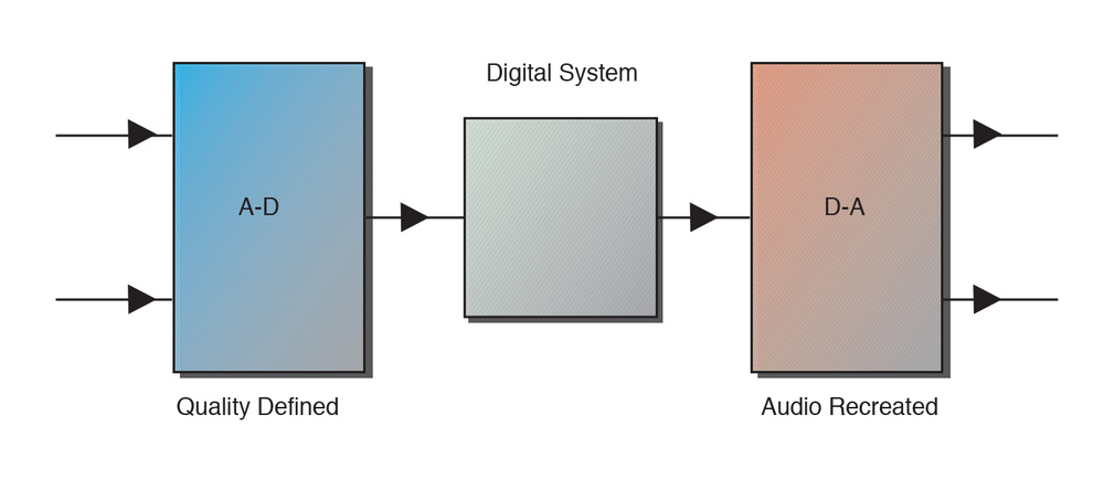
This fundamental characteristic of digital systems means that the quality of a digital audio signal is not primarily dependent on the physical medium used to store or transport it, but on the initial conversion from the analogue domain to the digital one, and the subsequent reconstruction to an analogue form for replay. The most important part of a digital audio system is the analogue‑to‑digital (A‑D) converter, because it is here that the audio quality is defined and fixed. If information is lost at this stage, nothing can be done to recover it later. One digital‑to‑analogue (D‑A) converter may make a better job of recreating the analogue signal from the digital data stream than another, but both are limited to working with the data as supplied by the initial A‑D conversion — which is why this first stage is so important (see Figure 2 on page 201).
Sampling & Its Side‑Effects
 DAT is a classic example of a digital medium designed for use by consumers that has ended up being used as a pro audio storage format.
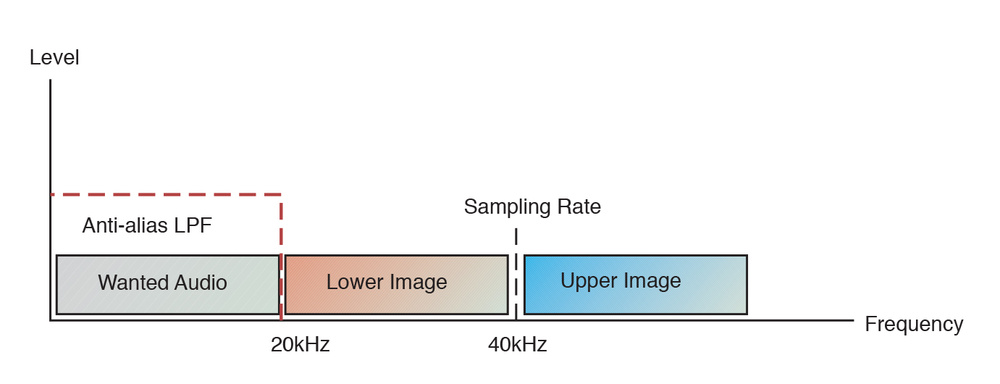
The process of sampling is in fact very similar to the amplitude modulation used in radio broadcasting on the AM bands. We needn't get into the exact details here, but suffice it to say that both processes produce artefacts known to the radio fraternity as sidebands. These are exact replicas of the original audio signal which mirror above and below the carrier wave or sampling frequency (see Figure 3 below). In digital audio circles these sidebands are usually known as images. The upper image is an exact replica of the original audio signal, but the lower one is an upside‑down version of it, with the lowest audio frequencies adjacent to the carrier, and the highest original audio frequencies transposed below.
These images are an inherent part of the sampling or amplitude modulation process, but the difference is that in radio broadcasting it is the sidebands which are detected by the receiver. By contrast, in digital audio applications, the sidebands serve no practical purpose and are merely an unwanted side effect. However, it is essential that the images do not interfere with the audio signal in any way, and they must remain separate from the original audio signal so that they can be removed without affecting the wanted audio. This implies that the sampling frequency must be selected so that the lower image and the original audio signal do not overlap at all. Figure 4 (below) shows how the full audio spectrum is replicated as images.
This fundamental principle of sampling was defined by a Swedish engineer called Harry Nyquist (working for the American Bell Telephone Labs) and is consequently known as the Nyquist Theorem. In short, the theorem states that in order to maintain separation between the highest part of the wanted audio signal and the descending image of it (the separation being necessary to allow removal of the unwanted images), the sampling frequency must be at least twice the highest audio signal. In other words, if a sampled audio system is required to carry signals from 20Hz up to 20kHz (supposedly the theoretical lower and upper limits of human hearing), then the sampling rate must be at least twice that — say 40kHz (as shown in Figure 4).
The important thing to note here is that by definition, in a sampled audio system we have to define and restrict the wanted audio bandwidth for it to work correctly — placing strict limits on what frequencies the system will pass and those it won't. This is a significant and important difference from a conventional analogue system.
Alias Filtering

As discussed earlier, raw analogue audio signals can contain a very wide range of frequencies — they don't stop at 20kHz just because we humans can't hear above that (if, indeed, many of us can hear as far up as 20kHz anyway!). We have also seen that we need to restrict the frequency range in a sampled audio system to comply with the Nyquist theorem. This implies that some severe audio filtering is required to restrict the upper frequencies being input to the sampling process, as well as to remove the unwanted image frequencies from the output signal.
If our sampling system operated at a 40kHz sampling rate and the original audio input happened to contain a signal at 30kHz (which would be inaudible to humans, but could still be present), the lower image of that signal would appear at 10kHz (See Figure 5 opposite). Not only would this be clearly audible, it would also be impossible to separate the unwanted image frequency from the wanted audio band.
This effect, where an unwanted signal appears in the wrong place, is called aliasing — and it sounds most discordant. The best description I can muster is that it sounds a little bit like the 'birdies' which can beset poorly aligned FM radio receivers sometimes — a kind of unrelated and unmusical chirping which, in extreme circumstances, can make the finest piano sound like a very rough harpsichord!
In analogue systems, distortion produces additional signals, above the original audio components, which are related harmonically — as in second or third harmonic distortion. These may be undesirable, but being 'musically' related to the source they tend to be acceptable — even beneficial — if sufficiently mild. However, aliasing in digital signals produces tones which are not musically or harmonically related to the source signals. Instead, they are mathematically related to the sampling rate and the aliases appear below the signal which caused them. Since this is a very unnatural phenomenon, the ear can detect aliasing even when there is only the smallest trace of it, and it is particularly unpleasant.
The visual equivalent of aliasing is strobing — the classic example being the wheels on the stage coach in an old western movie which appear to be going backwards slowly when in reality they are going forwards very quickly! The true rate of rotation is too fast for a film camera (with its slow 24 frames‑per‑second 'sampling rate') to capture, but the 'alias' of that rate is visible as a much slower, often reversed, rotation.
As it sounds so unpleasant, it is essential that aliasing is not allowed to occur in an audio sampling system, and the original analogue audio is low‑pass filtered to ensure that nothing above half the sampling frequency can enter the system. This filter is called an anti‑alias filter (since that is what it filters!), and it prevents the lower image and the audio signal from overlapping.
The sharpest low‑pass audio filters normally encountered on mixers or synths might have rolloff slopes of up to 24dB/octave, which means that for each doubling of frequency (ie. octave rise in pitch), the signal is attenuated by a further 24dB. However, to achieve sufficient isolation between the wanted audio signal and the unwanted lower image in a sampled signal, we need perhaps 90 or 100dB of attenuation for an anti‑alias filter — and there is typically only a fraction of an octave to do it in! Anti‑alias filters therefore have to be extremely steep, with rolloff slopes in the order of 200 or 300dB/octave, and in order to allow them sufficient space to achieve a useful degree of attenuation, the Nyquist theorem requires that the sampling rate is actually around 2.2 times the highest wanted audio frequency. (See Figure 6, above.)
As mentioned earlier, a very similar filter is required on the output of a digital audio system to remove ultrasonic images, left over by the sampling process, from the wanted audio signal. Although inaudible by definition, if left in place the very high image frequencies would quickly fry the tweeters of loudspeakers, could potentially cause instability in amplifiers or other electronic circuits, and would cause interference with the high‑frequency bias signals on analogue tape recorders. The output filter that removes these high frequencies is called a reconstruction filter and design economies usually mean that it is identical to the anti‑alias filter on the input of a digital system.
Assuming the anti‑alias and reconstruction filtering does its job adequately, sampling is potentially a perfect and reversible process. If the highest wanted audio frequency is known and spurious signals are correctly removed by the filtering, the wanted audio signal can be sampled and reconstructed without any loss in quality whatsoever. Unfortunately, however, nothing comes for free, and although the anti‑alias and reconstruction filters are an essential part of the signal path, they generate additional problems of their own!
The main problem with such unbelievably steep audio filtering is that it is extremely complex to design, and requires a large number of costly components. In the early days of digital audio these essential filters unfortunately affected sound quality rather badly as well, and were largely responsible for the hard, brash, fatiguing, and clinical sound originally associated with it. Fortunately, clever new techniques, such as oversampling and delta/sigma conversion, have evolved to get around these problems, and we'll look at these in detail next month.
Sampling Rates

The Nyquist theorem states that the audio sampling rate needs to be around 2.2 times the highest wanted audio frequency which, for a 20kHz system, would mean around 44kHz. Although there are arguments raging about whether 20kHz is a suitable upper limit for high‑quality audio systems, to employ a sampling rate higher than 2.2 times the highest wanted frequency is only wasteful of data capacity — it would provide no increase in information content because the anti‑alias filter restricts the audio signal to below half the sampling rate anyway.
As we all know, there are several common sampling frequencies in general use — there is a very apposite quip about the audio industry liking to establish standards... which is why there are so many of them! Broadcast, satellite and distribution systems typically use 32kHz sampling rates because traditionally the highest audio frequency carried on those systems was limited to 15kHz anyway. The lower the sampling rate, the less data there is to move about and so the lower the running costs — an important consideration in those applications.
The DVD audio lobby is pushing for 96kHz (and even higher sampling rates).
Commercial digital audio systems all operate on 44.1kHz — a value derived from the first videotape‑based digital recorders (see the 'Development Of Digital' box). That is why all pre‑recorded digital media operates at this rate:CDs, Minidiscs, DATs, laser discs, and DCC tapes, for example. A third rate, of 48kHz, was defined for so‑called 'professional' applications in the early '80s, but the reasoning behind this largely unnecessary and unhelpful sampling rate was quickly made irrelevant by advances in technology. Unfortunately, we are now stuck with it for the foreseeable future — especially in anything to do with digital video systems.
But why stop at 32, 44.1 and 48kHz? The DVD audio lobby is pushing for 96kHz (and even higher sampling rates) and the multimedia industry has used 22.05, 11kHz and 8kHz sample rates on computer games and the like for many years. There are also a host of very strange sampling rates, like 44.056kHz and 47.952kHz, which have evolved because of obscure incongruities between black and white and colour video frame rates in the American broadcast industry.
Coming Up...
 records to an internal hard drive, while the Tascam 654 uses Sony's compact Minidisc format.") These days, digital recording in possible to all kinds of media. The Fostex DMT8VL (above) records to an internal hard drive, while the Tascam 654 uses Sony's compact Minidisc format.
These days, digital recording in possible to all kinds of media. The Fostex DMT8VL (above) records to an internal hard drive, while the Tascam 654 uses Sony's compact Minidisc format.
Having got to grips with the basics of sampling, next month I will describe the process of converting the sampled audio signal into binary data (Quantising), the various problems encountered along the way, and how oversampling and delta/sigma converters have overcome some of these problems.
The Development Of Digital

Today's digital audio systems have evolved from technology first developed for the telecommunications industry, which in turn used ideas dating back to the early 1930s. The first professional audio applications materialised towards the end of the 1960s and early 1970s, when digital techniques began to offer substantial benefits over analogue setups in broadcast transmission and distribution systems. Analogue land lines were becoming prohibitively expensive and quality was relatively poor over long distances. Digital systems allowed costs to be reduced dramatically, whilst also improving reliability and sound quality into the bargain. Digital reverb systems followed in the late '70s, and at the time, these relatively small boxes of sophisticated electronics were far more cost‑effective and offered far greater flexibility than the huge echo plates and reverb chambers which were the previous best available technologies.
In the late '70s and early '80s, the march of digital recorders and players started with videotape‑based systems, initially in the professional CD mastering market. Although the off‑the‑shelf video machines used were grossly over‑engineered for the task of digital data recording, this approach did have the advantage that all the design effort could be put into making the analogue‑to‑digital and digital‑to‑analogue converters (crucial components in such systems, as explained elsewhere in this article).
At the same time, CD players proliferated and were later joined by DAT as an appropriately engineered replacement for the pseudo‑video systems. In recent years, we have seen the ranks of digital audio recorders swell enormously with the doomed DCC, the Minidisc, ADAT and DTRS digital multitracks, and countless magneto‑optical and hard‑disk systems. Digital signal processing is now commonplace, and digital mixers are increasingly gaining ground, both in the professional and project/home studio markets, as most SOS readers will be aware!
PCM — Pulse Code Modulation
Pulse Code Modulation is the form of binary coding used in virtually all digital audio systems. The name stems from the fact that it involves the 'modulation' or changing of the state of a medium (eg. the voltage within a circuit) according to coded blocks of data in the form of a string of binary digits.
PCM, as it is more commonly known, was invented in 1937 by a British engineer called Alec Reeves, but it wasn't until the electronics industry came up with the transistor that his idea became really useful. As usual, it was the telecommunications industry in the early '60s that developed the technique, eventually resulting in PCM as we use it today.
Home Truths — Cost Versus Quality
 Philips' DCC — a tape‑based digital format that failed to find the kind of pro audio niche that DAT did.
To the consumer and professional alike, digital audio systems are widely perceived to offer advantages over their analogue forebears in terms of audio quality, convenience of use and freedom from imperfections or degradation. Digital audio has an enormous dynamic range, a ruler‑flat frequency response, and no wow or flutter, and material is recorded onto compact media offering fast access times and an arguably long media life. However, the real reason digital audio systems appear to have overthrown their analogue equivalents in such a short period of time is because they are so inexpensive for a comparable level of performance.
Ten or more years ago, analogue audio components like record players and tape recorders had pretty much reached the pinnacle of their performance capability. The law of diminishing returns applied; it was simply not practical or cost‑effective to look for further improvements. A transcription‑standard record turntable today would probably cost somewhere in the region of £5000, and a Studer A80 stereo tape recorder could be as much as £12,000. Compare that to a professional CD player at £1500 (or less) or an all‑singing and dancing studio timecode DAT recorder at under £5000; it's no wonder that the analogue audio industry is rapidly fading into the background!
Whereas the best analogue audio recorders and players employ relatively simple electronics, they require extremely well engineered (and thus very costly) mechanical transports. Digital techniques allow remarkably simple, low‑cost mechanics to be used with exceptionally complex electronics which recover the digital data, remove any degradations and provide 'perfect' replay! Designing and developing the digital electronics is extremely expensive, but mass production means that the cost per unit can be extremely low. Hence the enormous price advantages of digital audio equipment over analogue — particularly in the consumer markets, where the sales volume is so vast.
The inherent knock‑on from this is that whereas domestic audio equipment used to derive from professional designs, these days most R&D effort is focused on the high‑profit consumer sectors. Consequently, professional equipment is now largely derived from domestic designs — the DAT being the most obvious example.
Of course, this kind of technological progress is not confined to the audio industry. If you wanted a fast car in the 1930s, the engine would probably have had 16 cylinders, an enormous capacity, and (by today's standards) an unbelievable thirst for petrol. These days, a tiny 1.1‑litre turbo‑charged engine can generate twice the power with far less fuel, but relies on a very sophisticated digital engine management system to stop the thing from blowing itself to bits!
Binary Bits & Pieces
The decimal number system (ie. based on units of 10) is a very convenient counting format for humans because we have 10 fingers, but binary is far better suited to machines, where simple on/off, yes/no states prevail. Binary numbers exist in one of two states, so instead of counting from 0 to 9, binary counts from 0 to 1.
In decimal, once a count of nine is exceeded, another digit is required. The digit in the right‑hand position of a number — the seven in 367, for example — represents the units, the number to the left represents the tens, and the one on the left of that, the hundreds. Each further digit added to the left increases the count by ten times — thousands, ten thousands, hundred thousands, millions, and so on.
In binary, each additional position to the left of the first digit increases the value in factors of two — units, twos, fours, eights, sixteens and so forth.
| DECIMAL units |
BINARY 4s/2s/units |
| 0 | 000 |
| 1 | 001 |
| 2 | 010 |
| 3 | 011 |
| 4 | 100 |
| 5 | 101 |
| 6 | 110 |
| 7 | 111 |
Although binary is a very convenient format for machines, it has its own inefficiencies; it requires roughly three times as many digits as decimal to represent a large number. Fortunately, the advantages of binary outweigh this minor disadvantage — even if it does mean that we end up with some very large strings of binary numbers. Most current digital signal processors manipulate 32 bits at a time, and that number of digits can represent the equivalent of over four billion in decimal — plenty big enough for most audio applications!
Each number in the binary sequence is called a bit — a contraction of Binary digit. The number on the extreme right representing units is called the least significant bit (or LSB) and the one on the extreme left representing the highest multiplier is called the most significant bit (or MSB) — terms you may well have encountered before without knowing what they mean!