Our second instalment draws on the work of Alan Blumlein, to explain how we can audition and evaluate different stereo‑miking techniques.
In Part 1 of this series on stereo miking techniques we looked at the intentions behind recording in stereo, and how the human ears/brain work out the location of an audio source in the real world, using three primary mechanisms: inter‑aural level differences (ILDs), inter‑aural timing differences (ITDs), and spectral cues from the sound reflections off the shoulders and pinnae. The reason we needed that background information is that, when we capture and replay stereo recordings, our aim is to recreate those auditory locational cues, either as accurately as possible, or in a way that is pleasingly believable.
So, before moving on to examine different stereo microphone techniques, we need to consider how the ways in which we audition two‑channel stereo recordings emulate the real‑world experience. And for that, we need to look in particular at the pioneering work in the 1930s of Alan Dower Blumlein.
Until such time as humans can be upgraded with direct Bluetooth reception to the auditory processing centre in the brain, we only have two options for listening to stereo recordings: loudspeakers or headphones/earbuds. Both approaches have their merits and disadvantages, but they each interface with the human hearing system in dissimilar ways, so result in significantly different experiences.
By their very nature, headphones (and earbuds) isolate each ear, which can only hear the signal presented via its own channel. This is in contrast to real life where both ears always hear a sound source with different levels, timings and frequency responses, as previously explained. So, this aural exclusivity is inherently unnatural, and the most obvious result is sounds being perceived as existing within the head — along an imaginary line between the ears, rather than in the space around us. There are ways to resolve that problem, though, and I will return to that in the future.
In the meantime, listening over loudspeakers is where stereophony began, and the majority of stereo microphone configurations are optimised for this format... so that’s where I’m going to start.
Loudspeaker Stereo
To most people, ‘stereophonic’ implies two loudspeakers, but it wasn’t always that simple. Back in the early 1930s, Dr Harvey Fletcher and his team, working for Bell Labs in America, were experimenting with multi‑channel sound recording and reproduction. His initial work used a large curtain of many microphones, arranged laterally and vertically in front of a stage, effectively sampling the combined sound wavefront projected from an ensemble on that stage. Each of those microphones was linked individually (via suitable gain stages) to a correspondingly located loudspeaker in a separate listening room, the idea being to reconstruct the original sound wavefront, preserving all directional information from the sound sources on stage — a system which was known as the ‘Curtain of Sound’.
 Fletcher’s Curtain of Sound.
This system actually worked very well, but of course it was highly impractical — especially since multi‑channel recording and transmission hadn’t yet been invented, from the recording and transmission points of view! Fletcher and his team therefore simplified the system, eventually deciding that three microphone/loudspeaker channels, arranged as left, centre and right, in a horizontal line, was the minimum arrangement for recreating acceptable locational information.
To demonstrate this new format to the public in March 1932, Fletcher arranged a live relay, using telephone lines to route the three audio channels from the Academy of Music in Philadelphia to the Constitution Hall in Washington. The Conductor in Philadelphia was Leopold Stokowski, who had a great interest in improving recorded sound, and he went on to help Disney develop its bespoke surround‑sound system, Fantasound, which was launched in a roadshow tour of the Fantasia film to public theatres across the USA in 1940.
The results of Fletcher’s public demonstration were considered impressive, but the technical difficulties of managing even three channels — maintaining their critical phase, timing and level relationships — eventually curtailed further development. From a commercial perspective, another significant problem was how to create a mono recording for release on a 78rpm disc. Downmixing all three mic channels to mono resulted in unpleasant comb‑filtering, while only using the centre channel lost information from the sides, compromising the overall balance. Solutions were found in time, of course, most notably with the superb Mercury Living Presence recordings made by Robert Fine in the late 1950s and early ’60s.
Blumlein... realised that recreating the original source time‑of‑arrival differences from three loudspeakers, as Fletcher was doing in America, had serious inherent problems.
Meanwhile, in early‑1930s UK, Alan Blumlein was working for EMI on sound recording and reproduction techniques, and he realised that recreating the original source time‑of‑arrival differences from three loudspeakers, as Fletcher was doing in America, had serious inherent problems. Chief amongst these is that both of the listener’s ears can hear signals from all the loudspeakers. Consequently, the intended time‑of‑arrival differences captured by the stage microphones were subsequently confused by the additional time‑of‑arrival differences created by each of the replay loudspeakers. Moreover, these additional ITDs are dependent on the position of the listener relative to the speakers, making life difficult in theatre settings with lots of listeners.
It occurred to Blumlein, though, that this apparent problem of each ear hearing all loudspeakers could potentially be used to advantage — but only if he gave up the idea of capturing the real time‑of‑arrival differences from the sources. This new scheme relied on reproducing only intensity (amplitude) differences between the signals feeding each loudspeaker, a system which creates an illusion of directional sound information with remarkable realism and stability. He called his invention Intensity Stereo. To work with reasonable accuracy, it requires the speakers and listeners to be positioned at the points of an equilateral triangle (ie. with a 60‑degree listening angle). This arrangement fools the ear/brain into translating the pure level differences between signals from the two loudspeakers into artificial ITDs, portraying spatial information about (virtual) sound source positions arrayed between the two loudspeakers. This brilliantly clever solution is explained in the ‘Stereo Illusion’ side box.
It is worth noting in passing, though, that Intensity Stereo is not the only way to create the impression of different spatial positions. A similar effect can be created by introducing small delays into signals of identical levels reproduced from each loudspeaker — something I’ll come back to later.
Coincident Microphones
Having come up with a workable system to create the illusion of virtual sound sources positioned in space between a pair of loudspeakers, the logical next question was how to capture the positioning of real sound sources on a stage and convey that information to the loudspeakers as an Intensity Stereo signal.
The critical aspect here is that timing differences between the channels are expressly not required, so separate, spaced microphones like Fletcher was using are not acceptable. Instead, the two microphones feeding the two channels must receive all sounds at exactly the same time, and that means they must occupy the same point in space — in words more familiar to recording engineers, they must be coincident in space. Also, to create suitable amplitude differences in each channel proportional to source stage positions, the microphones require directional polar patterns, and to be aimed in different directions.
In the 1930s, microphone polar pattern options were relatively limited, with figure‑eight ribbon mics being the best option for Blumlein’s coincident microphone experiments, resulting in the stereo mic array that has acquired his name. The Blumlein array comprises two figure‑8 mics mounted vertically, one above the other, such that they are coincident in the horizontal plane. One mic is typically arranged to face 45 degrees left, and the other 45 degrees right, such that the mutual angle between them is 90 degrees (although other options are available and I’ll discuss them next month).
 The classic Blumlein array has an SRA of 76 degrees.
A central sound source in front of these coincident microphones will be captured at the same time and the same level (albeit off‑axis) in both, thus creating a central phantom image when auditioned on loudspeakers. If the sound source moves to the left, it will move more on‑axis to the left‑facing mic, and more off‑axis to the right‑facing mic, thus creating a level difference between the two channels, being louder on the left. This level difference creates a corresponding image position when heard on loudspeakers.
When the sound source is directly on‑axis to the left microphone, it will also be directly in the null of the right microphone, so virtually all the signal will be in the left channel (ignoring any reverberation) and the sound will therefore emanate only from the left loudspeaker. So, this arrangement creates a stereo recording angle or ‘SRA’ in front of the microphones — a region being recorded which is effectively ‘mapped’ into the available space between the two loudspeakers during replay. In the case of the Blumlein array as described, that SRA is about 76 degrees, but every different stereo mic array will have a specific SRA value. Again, much more on that in Part 3, but for now, this SRA value matters because the sources you wish to record have to be contained within the mic array’s SRA if they are to be portrayed with reasonably accurate relative locations from the loudspeakers.
Listening
To illustrate the strengths and weaknesses of different stereo mic arrangements I’ve prepared a series of demonstration recordings that you can find on the SOS website (https://sosm.ag/this-is-stereo-media). Over about an hour on a warm summer’s evening, I recorded the Teme Valley South Churches Choir (TVSCC), founded and conducted by Chloe May Evans, in a hilltop church in Worcestershire, UK. I am immensely grateful for their generosity and patience as this required them to perform the same piece repeatedly in front of a number of different mic arrays, some being reconfigured and/or physically moved between takes!
, who kindly repeatedly performed ‘If Ye Love Me’ by Thomas Tallis, to help us demonstrate the different stereo mic arrays.") The Teme Valley South Churches Choir (TVSCC), who kindly repeatedly performed ‘If Ye Love Me’ by Thomas Tallis, to help us demonstrate the different stereo mic arrays.
The Teme Valley South Churches Choir (TVSCC), who kindly repeatedly performed ‘If Ye Love Me’ by Thomas Tallis, to help us demonstrate the different stereo mic arrays.
I shall describe more of these recordings, and their specific points of interest, in future articles but, for now, I suggest that you listen to the first track, which was captured with a Neumann SM69 FET single‑bodied stereo mic set up as a Blumlein array of figure‑8s with a mutual angle of 90 degrees. The Blumlein arrangement captures sound from the mics’ rear lobes in addition to the front ones, which adds to the overall room reverberation, while reverberant sound arriving at the sides is captured in opposite polarities by both mics, adding to the sense of spaciousness. Although not apparent here — the small choir were positioned in a single line — this particular mic array is also particularly good at portraying stage depth in a realistic manner.
In the next article, I’ll continue to explore coincident mic techniques, compare their strengths and weaknesses, and look at some useful practical tools for choosing and optimising different arrays.
Stereo Illusion
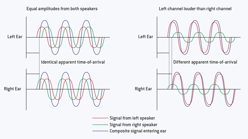
Blumlein’s revolutionary invention of Intensity Stereo is ingenious, but the concepts can be explained simply by considering steady sine‑wave tones being reproduced by each loudspeaker — yes, I realise that I said in Part 1 of this series that it’s hard to locate steady tones in real life, but it’s much easier to follow the theory if we use sine waves! Let’s start with an identical sine tone reproduced at identical levels by both loudspeakers, as illustrated in the diagram above. The left ear receives the signal from the (closer) left speaker first (red wave) and then from the right speaker (green wave) a short time later.
The reverse happens in the right ear, of course, but, since the listener is at the apex of an equilateral triangle, with the speakers at the other two points, the distance between right ear and right speaker is the same as the distance from left ear to left loudspeaker. Consequently, the right speaker signal arrives at the right ear at exactly the same time as the left speaker signal arrives at the left ear. A few microseconds later, each ear hears sound from the more distant speaker.
Now, the two signals arriving at each ear will sum together acoustically as they arrive at the ear drum — that result is shown as the blue wave for each ear. As the signals from both loudspeakers have identical levels, the resultant signals entering each ear will be identical, and its apparent starting time is exactly mid‑way between the real signals from each speaker. So, as far as the ear and brain are concerned, these two resultant signals (blue) have exactly the same time‑of‑arrival at both ears. Therefore, the virtual sound source is perceived to be directly in front of the listener — a ‘phantom’ central sound source.
If we now alter the relative levels of the signals produced by the two loudspeakers, which is easily achieved using a pan pot, for example, something rather magical happens. The illustration on the right shows that the signal from the left loudspeaker (red wave) is now much louder than that from the right (green wave).
When these signals combine as they enter the ear, the louder one dominates the sum, so the resultant signal appears to arrive earlier in the left ear than it does in the right. Again, as far as the ear/brain are concerned, we detect an ITD, which we perceive as a sound source to the left of the listener — its exact position is dependent only on the relative levels of signals from the left and right loudspeakers. As a rough guide, a level difference of 16dB is sufficient to create the illusion that a sound source is located firmly at a loudspeaker, while a 4dB difference moves the source from the centre to about a quarter of the way across from the centre towards the louder speaker, 8dB about half‑way, and 12dB about three quarters of the way.
In other words, relative level differences (ILDs) between the signals reproduced by two loudspeakers are translated automatically into time‑of‑arrival differences (ITDs) at the ears, creating the illusion of virtual sound sources spread across the 60‑degree angle between the two loudspeakers.
Naturally, there are physical limits to the creation of stable stereo imaging, and the most obvious occur if the listener moves away from the apex of the equilateral triangle — the listening sweet spot, as we sometimes call it. Staying central but moving further back reduces the perceived ITDs, so the stereo image narrows. Conversely, moving forward, inside the triangle, increases the ITDs. This stretches the image wider, but also makes the phantom centre unstable. Moving to the left or right greatly exaggerates the perceived ITDs, and eventually the Haas effect takes over, whereby the brain latches onto the sound source it hears first — the nearest loudspeaker — and the stereo imaging collapses into the single speaker.