

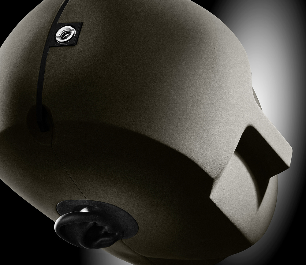
Concluding our series on advanced stereo mic techniques, we explore binaural recording, disc‑shaped baffles and dummy heads, as well as a clever process called ‘Stereo Shuffling’.
The preceding parts of this series took us on a journey from the fundamental concepts of stereo sound recording and reproduction to the theory and practical aspects of a wide range of stereo microphone techniques. We’ve explored Blumlein’s coincident arrays, including Mid‑Sides, that focus on capturing and reproducing only amplitude differences between channels; and the wide‑spaced omni‑mic arrays that capture mainly time‑of‑arrival differences between channels. We went on to consider a number of popular near‑spaced arrays that were designed to combine both amplitude and timing differences between channels — the best of both worlds — before also contemplating some of the more complex stereo mic arrays that combine both spaced omnis and near‑spaced arrays, including a brief look at the famous Decca Tree.
By this point, then, you’d be forgiven for thinking that there couldn’t possibly be any more stereo mic arrays to examine! But there are — and if you’ve been working through the audio example files associated with this series, you’ll already be aware of one example: the Schneider Disc. This, with variations upon it, is the last stereo mic array that I want to discuss in this series, as it represents a final class of stereo microphone techniques that aim to replicate the human hearing physiology — to a greater or lesser extent.
Dummy Head
If the idea of stereo recording is to replicate the human experience of listening to performers on a stage, arguably the most obvious approach is to imitate the human listening apparatus. Basically, that means using a head‑shaped construction with microphones in place of the ears. This concept, popularly known as the ‘dummy head’, has been explored in depth for decades, and there are several commercial examples, including Neumann’s original KU80 and current KU100, and Sennheiser’s now discontinues MZK2002, amongst various others.
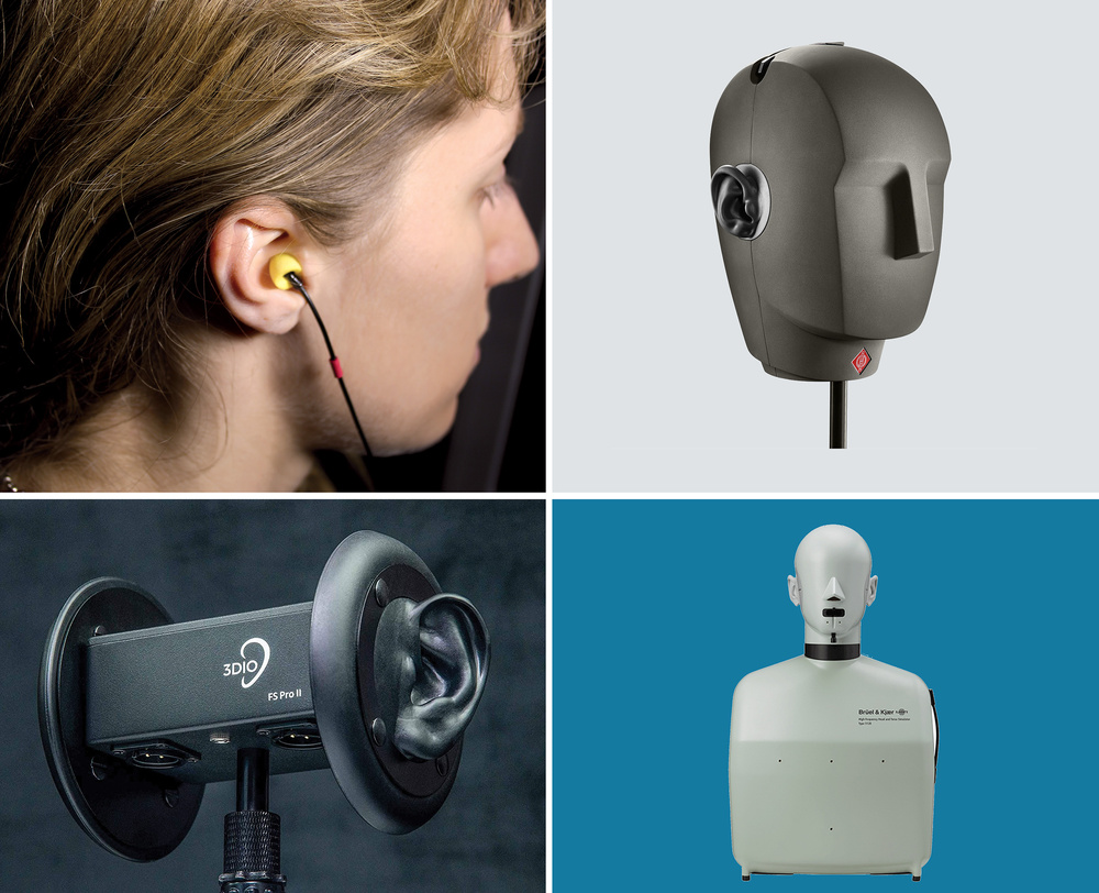
A range of mics intended to replicate the human listening experience. Clockwise from top right: the Neumann KU100 dummy head; Bruel & Kjaer’s HATS system; the 3DIO FS Pro II; and some ear‑worn mics. The last of these could potentially be the most convincing — but only for the person who wore the mics!
These dummy head systems produce a stereo signal in a format generally referred to as ‘binaural’, and intended exclusively for headphone listening. However, the success of these dummy head recordings, in terms of imaging stability and source location realism, depends very heavily on how closely the listener’s anatomy matches that of the dummy head, particularly in terms of head size and ear spacing (early dummy heads don’t attempt to replicate the folds and curves of the pinnae which, as we know, play an important role in vertical and front/back source location). The physiological parameters of the listener’s head/ears determine what is now known as the ‘Head Related Transfer Function’ or HRTF, which is unique to each individual listener, and it is these parameters that define how we individually perceive sound locations within a binaural signal.
As it happens, I own a Sennheiser MZK2002 dummy head. The recordings I’ve made with it certainly sound spacious and are interesting, but I don’t find them consistent, stable or precise. That’s probably in large part because the dummy head is physically smaller than my own. If I attach the same Sennheiser microphones to my own ears for recording, then playing back the audio files gives me remarkably precise and stable imaging information. But it’s important to note two things... First, if you move your head at all, you change the perspective of the mics. And second, this approach benefits me alone — others who’ve listened to recordings I’ve captured that way usually find the imaging to be imprecise and unstable again. This highlights the critical importance of personal HRTFs for accurate spatial imaging in binaural listening.
Today, of course, there’s a huge academic and commercial interest in binaural stereo, not least because of the vast numbers of people who now listen over headphones habitually. And while personalised binaural recordings might not transfer well from one listener to another, binaural reproduction is an ideal format for low‑cost immersive‑audio playback. Indeed, with the benefit of sophisticated digital signal processing, and the ability to create and implement personal HRTFs for playback over headphones, binaural stereo is making significant headway in popularity, and many manufacturers are now incorporating this technology in smartphones, tablets, laptops and more.
One down side of binaural stereo and dummy‑head recordings is that the format is specifically intended for use with headphones, and the stereo imaging is usually very poor when heard over loudspeakers.
One down side of binaural stereo and dummy‑head recordings, though, is that the format is specifically intended for use with headphones, and the stereo imaging is usually very poor when auditioned over loudspeakers. That wouldn’t be a problem if the entire audience were known to use headphones, but in most cases a significant proportion of the audience for commercial music is likely to be listening over loudspeakers. So is there an alternative technique that could offer better compatibility between headphone and loudspeaker listening?
Optimal Stereo Signal (OSS)
Take away the physical differences between individuals’ heads and ears, and the main significance of the replica head in dummy head recordings is that it acts as an acoustic baffle, reducing the strength of high frequencies from a source on one side reaching the ear on the opposite side, as well as introducing a time delay to the further ear. So why not just reduce the ‘dummy head’ to its simplest form: a flat baffle, with microphones placed on either side?
Needless to say, it’s been done... and as you might already have guessed, the first person to do it was Alan Blumlein, back in the early 1930s. One of his earliest experiments involved a pair of pressure (omnidirectional) mic capsules separated by an acoustic baffle. He described the setup in his famous patent, along with sophisticated signal processing to make it work better for loudspeaker listening, which is something I’ll come back to shortly. It wasn’t a line of enquiry Blumlein pursued at the time, though, as he chose instead to focus his work on coincident velocity (directional) microphones, which, to his mind, gave better results with loudspeaker auditioning. But good ideas have a habit of resurfacing sooner or later, and it was the work of Jürg Jecklin in the early 1980s, at the University of Music and the Performing Arts in Vienna, that resurrected the interest and popularity of Blumlein’s idea. He called the technique the Optimal Stereo Signal or OSS — but it became far better known for its physical appearance, and is usually referred to simply as the Jecklin Disc.
Jecklin Disc
Jecklin’s earliest design employed a flat, 30cm diameter disc, covered in a thin layer of foam (or fleece) to reduce the baffle’s acoustic reflectivity. A pair of omnidirectional microphones were then mounted on either side of the disc, their capsules being aligned with the centre of the disc, spaced 16.5cm apart (so roughly 8cm above the disc’s surface) and pointed outwards by 20 degrees.
In essence, the disc baffle broadly replicates the primary acoustic effects of the human head, with the baffle diameter and mic spacing combining to introduce similar frequency response, time and amplitude differences between the two microphone signals as are experienced at the ears of a listener. Those differences increase as a sound source moves further off axis from the front of the disc, much like it does with human hearing.
Most commercially made OSS discs follow Jecklin’s original specifications for the baffle size and mic spacing, but in the mid‑1980s Jecklin himself revisited the design, and concluded that it performed better with a larger baffle diameter and greater mic spacing. Consequently, he issued revised specifications, with a disc diameter of 35cm, and mic spacing increased to 36cm (so roughly 17cm above the disc surface).
Commercial Jecklin Discs are not inexpensive, but anyone handy at basic DIY can construct their own experimental Jecklin Disc relatively easily, using something like a piece of plywood or Perspex cut into a disc. While the size/diameter is fairly important, you don’t even need to be able to cut a perfect circle (the human head is broadly ellipsoid rather than spherical, after all). A handle or mic stand mounting thread can be attached to the disc, along with a pair of threaded studs or tubes mounted near the back to support standard mic clips. Their positioning needs to accommodate the length of the intended omni mics such that their capsules end up near the centre of the disc when angled outwards by 20 degrees. The plywood or Perspex disc casts an acoustic shadow, but as it also reflects sound, it can then be covered with some acoustic foam and/or fleece on each side. Then your Jecklin Disc is ready for use!
Schneider Disc
As always when it comes to stereo mic techniques, there are several variations on this theme, and the example (track 10) audio recording included in the audio files associated with this series (https://sosm.ag/this-is-stereo-media) was captured using what’s known as a Schneider Disc, a version of the OSS technique that’s very similar to the standard Jecklin Disc. The baffle diameter is the same as the original Jecklin specs, and the mic spacing is the same too. However, in addition to the flat layer of foam on each side of the baffle, a hemisphere of foam is added at the centre of the baffle on each side. The idea of this extra foam is to better replicate the acoustic absorption effects of the human head. To be honest, the audible difference between a Schneider Disc and a Jecklin Disc is very subtle. My own view is that the Schneider version performs slightly better, particularly for headphone listening, but there’s really not a lot in it! (If going down the DIY route suggested above, you could always conduct your own experiments with different absorptive material...)
In the foreground is the Schneider Disc array (a variation on Jecklin’s original OSS technique) used for example 10 in the audio recordings that accompany this series.
Jecklin recommends that the ideal placement of the (Jecklin or Schneider) Disc is at the room’s ‘critical distance’ (Dc) away from the source — where its direct sound and diffuse (reflected) sound are equal in strength. Personally, I prefer a slightly closer placement in most cases, but that’s an aesthetic choice, and one that depends on the nature of the music and source, and the sound perspective required. For the Schneider Disc demonstration in the associated audio files, I mounted a pair of Sennheiser MKH20 omnidirectional mics on the disc, spaced roughly 17cm apart with the disc positioned just above head height, and (because it was a particularly reverberant church, making the Dc distance relatively short) around 2.5 metres in front of the choir.
I have enjoyed good results using the Schneider Disc on small ensembles, particularly if the main audience is likely to be headphone users. However, the OSS system also works nicely as a main stereo array for larger ensembles, with excellent bass extension and a nice spaciousness that still works reasonably well on loudspeakers. The recording setup always attracts attention at public concerts, too (not because it’s particularly obtrusive; it’s more that people don’t see it used very often so are curious).
Stereo Shuffling
One of the reasons Blumlein didn’t pursue his baffled‑omni‑mics idea was because it didn’t generate purely level differences between the two channels at all frequencies — you’ll recall from earlier articles in this series that accurate stereo imaging from loudspeakers primarily relies on reproducing only amplitude differences between the two channels.
For off‑axis sound sources, the baffle placed between the omni mics naturally introduces amplitude differences between channels at mid and high frequencies (where the wavelength approaches the baffle diameter). However, at lower frequencies the soundwaves simply diffract around the baffle, resulting in negligible amplitude differences between the two omnidirectional mics. Thus, low‑frequency sources appear to come from the centre of the stereo image, with negligible stereo width.
Nevertheless, the mics capture some low‑frequency directional information because their physical spacing generates small phase differences at low frequencies, due to the different time‑of‑arrival of sound wavefronts at each mic. In an attempt to improve low‑frequency stereo imaging over stereo loudspeakers, Blumlein developed a method of converting those low‑frequency phase differences between channels into representative amplitude differences, and named this process Stereo Shuffling. As I mentioned earlier in this series, this Shuffling term has been used in a few different contexts and applications over the years, and that’s naturally led to confusion in some quarters! But the underpinning concept of all Shuffling processes is that they provide a frequency‑dependent stereo‑width correction.
Blumlein’s original Stereo Shuffling system worked in three distinct stages. First, the left‑right stereo signal from the microphones was converted into the Mid‑Sides format. Second, the amplitude of low frequencies in the Sides channel only was boosted, typically by around 8dB below 600Hz, using a first‑order (6dB/oct) low shelf. Finally, the processed result was converted back into left‑right stereo. This frequency‑conscious Mid‑Sides processing cleverly converts the small phase differences between channels into significant amplitude differences, thus allowing much better stereo imaging when heard over loudspeakers. The size of the baffle determines the frequency above which the mics capture amplitude differences between channels and, for a head‑sized baffle, that’s above about 600Hz; below that it’s just phase differences — hence using that frequency as the corner of the shelf EQ.
Other Shuffling Applications
As we’ve seen in previous articles in this series, various other stereo mic arrays also have inherent frequency‑dependent stereo image width issues, and the same Shuffling concepts can often be used to help correct or improve the stereo imaging for loudspeaker listeners when using those recording systems. I mentioned in Part 3, for example, how Stereo Shuffling can be employed to correct the tendency of directional mics to lose their directionality at low frequencies in coincident arrays, and how it can also compensate for the high‑frequency beaming associated with figure‑8 ribbon mics in a Blumlein array. The same technology also works particularly well with the Gerzon array, for example, which I described in detail in SOS November 2020 (https://sosm.ag/the-gerzon-array).
One ‘problem’ with the Shuffling process is that, unless using a linear‑phase EQ, phase‑shifts occur whenever an EQ circuit is used (so it’s inherently an issue when implemented in analogue circuitry). If only the Sides signal is processed, that path incurs phase‑shifts that aren’t replicated in the Mid path, and when the two signals are recombined to produce left‑right stereo those phase‑shifts can affect the overall tone in unhelpful ways.
In the case of the Gerzon array, the Sides channel bass boost EQ used in the Shuffling correction introduces around 25 degrees of this ‘phase lag’ at 600Hz. That’s a part of the spectrum where human hearing is relatively sensitive to phase shifts. Fortunately, the 5cm capsule spacing employed in that array introduces a similar amount of ‘phase lead’ in the (converted) Sides channel, effectively counteracting the effect and minimising any phasiness in the processed and decoded output.
If applying Shuffling in a DAW, one can of course choose to use linear‑phase filters in the Sides path. These don’t introduce frequency‑dependent phase‑shifts, but they will inherently introduce latency. Modern DAWs can correct that automatically on playback, but if they don’t (for example if you choose to bypass automatic latency compensation while recording), there may well be obvious comb‑filtering artefacts in the decoded left‑right output. Sometimes, applying a complementary cut in the Mid channel to balance a reduced boost in the Sides channel can give better results than processing only the Sides channel.
It’s fun and also educational to construct Stereo Shufflers in the DAW from a combination of M‑S matrix and EQ plug‑ins — and there are plenty of EQs that can act separately on the Sides signal now of course. I’d encourage you to experiment with the amounts of boost (or cut) and the corner EQ frequencies — there are no rules, only good or bad results!
You can recreate the stereo shuffler effect in your DAW, either by putting an EQ between Mid‑Sides encoder and decoder, or by using an EQ plug‑in that allows you to process the Sides signal separately.
If you’re looking for an easier life, Pspatial Audio’s Mac‑only Stereo Lab 4+ software contains myriad stereo processing tools intended for 78rpm records, modern RIAA vinyl, CD de‑emphasis, tape and cassette processing, headphone enhancement, surround upmixing, and much more. It also includes a number of different Shuffler configurations, including modes optimised for coincident figure‑8 and cardioid mics, as well as several variations on Stereosonic shuffling to improve loudspeaker monitoring. I highly recommend it.
For real‑time Shuffling, there’s Phaedrus Audio’s SHUpHLER, the original version of which I reviewed in SOS July 2017. The latest version of this compact unit can be switched between several different Shuffler configurations, mostly the same as found in Stereo Lab, albeit without the linear‑phase models. It processes the audio entirely in the analogue domain for real‑time applications. Blumlein’s Shuffler for baffled spaced omnis is called Blumlein δ (delta) and it can be used on most near‑spaced stereo mic arrays with good results. An alternative Shuffler, marked with an inverted heart symbol, has been optimised for coincident cardioids, but can also be useful with near‑spaced cardioid arrays. The entertainingly named Bride Of Francinstein Shuffler is a modern take on EMI’s Stereosonic Shuffler, to help correct for the inherent stereo imaging compromises of loudspeaker listening. A fifth mode provides a straightforward Mid‑Sides matrix.
Phaedrus Audio’s SHUpHLER, based on Blumlein’s Stereo Shuffler idea, can restore to recordings the sense of low‑frequency stereo definition that’s often lost on loudspeakers.
Stereo Width Adjustment
When I discussed the Mid‑Sides stereo mic array in Part 4, I explained how changing the relative balance of the Mid and Sides channels altered the effective Stereo Recording Angle (SRA). In exactly the same way, if a left‑right stereo signal is converted to Mid‑Sides, adjusting the Mid:Sides balance alters the width of a decoded stereo signal when auditioned over loudspeakers. This is a very useful facility that’s built into the stereo channels of some sound consoles, and most DAWs include a stereo width plug‑in (if not, try Voxengo’s freeware MSED) that can be used for the same effect.
Altering the stereo width in this way with material created using pan‑pot stereo or a coincident stereo mic array source is inherently problem‑free; there are no adverse stereo imaging side‑effects to worry about unless the Sides signal is increased too much, resulting in a very out‑of‑phase sound with a hole in the middle of the image. A phase meter or stereo vectorscope is the ideal visual aid to ensure the stereo width stays within sensible limits! Introducing an equaliser into the Sides channel, to increase the stereo width below about 600Hz, generally has a very beneficial effect on the sense of spaciousness in a recording — another use for Shuffling!
However, increasing the stereo width in this way with near‑spaced stereo mic array sources can introduce significant problems, and should be used with great care. The fundamental problem is that, as the microphone capsule spacing inherently introduces significant phase‑shifts between the two channels, at a certain frequency (and its higher harmonics) the phase‑shift will approach 180 degrees. Because the Mid‑Sides conversion involves sum‑and‑difference processing, those frequencies will create deep notches or peaks in opposite channels in the decoded stereo signal. So, while increasing the proportion of the Sides signal relative to the Mid will increase the stereo width at low frequencies, it will also alternately narrow and widen the signal at higher frequencies, potentially resulting in a substantially degraded and confused stereo image!
The only way to avoid this problem with near‑spaced arrays is to restrict any stereo widening effects to the lower frequencies, where the phase‑shift gets nowhere near 180 degrees. The maximum Sides channel turnover frequency that can be safely used can be calculated from: Hz = 5400/d.
In this equation, d is the capsule spacing in centimetres. So, for example, the highest acceptable frequency for stereo‑width enhancement of an ORTF array is 317Hz (5400/17). For an NOS array it would be 180Hz... and so on. The wider the capsule spacing, the lower the safe processing frequency. That said, with very widely‑spaced mics (say, over 1.5 metres) the signals in the two channels are so highly decorrelated that the phase‑cancellation of higher frequencies ceases to be a problem.
To sum up, then, using Mid‑Sides processing to change the width of a stereo signal works well with coincident mic recordings and with pan‑pot stereo material, where there are no significant phase differences between channels. But, where there are deliberately introduced phase differences due to microphone capsule spacing, stereo widening should be applied with great care, paying attention to the stereo imaging of the mid and higher frequencies, which may become excessively wide or narrow. If this occurs, restrict the width enhancement to the lower frequencies only according to that formula above.
That’s All Folks!
With that, here endeth our series of lessons on practical stereo microphone techniques. Along the way, I’ve tried to point you to several other resources that I’ve found very helpful, and there are plenty more available on the web and in the bookshops — and some will include details on some more esoteric arrays, such as the Double Mid‑Sides array and the Blumlein‑Pfanzagl‑Triple array that might well be worth exploring if you want to journey further down this road. Hopefully, though, this series has helped to demystify many aspects of stereo miking. I also hope this series will encourage you to experiment more confidently with a greater range of techniques. Remember that there really are no rules, just options: the end results are all that matter — and armed with an understanding of the benefits, possible pitfalls and potential for modification of different arrays, you should be able to capture exactly the results you desire. Happy recording!

